How to create a graphical return comparison
See also:
Other use case examples:
- How to create cumulative returns using the Quintessence Excel® Addin functions
- How to build formulas in Excel using the Quintessence Excel® Addin functions
How to create a graphical comparison between a portfolio’s returns and an index
The goal is to compare the performance of a fund against an index over a period of time, and to create a graphical representation of the differences.
The workbook will have three sheets: a configuration sheet, a data sheet and a graphics sheet. The configuration sheet will contain a list of portfolios. These will be used to create a lookup selection list. The data sheet will contain the data function calls that retrieve information from the database. The graphics sheet will contain graphs and calculations.
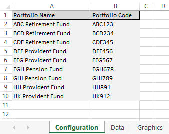
Create a list of portfolios
Create an Excel workbook with three sheets called ‘Configuration’, ‘Data’ and ‘Graphics’. On the first sheet, list a set of portfolio names along with their codes:
Create the selection ‘dashboard’
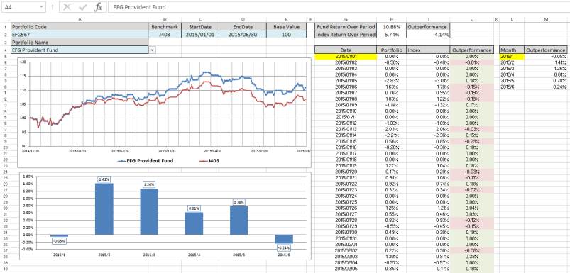
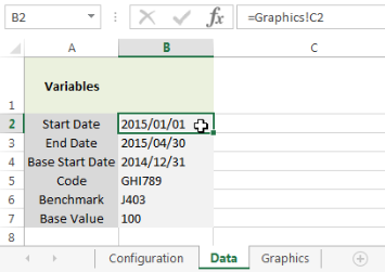
On the ‘Graphics’ sheet, create entries for the benchmark index, start date, end date, a base value for the cumulative returns, and a portfolio code lookup. These dashboard values (benchmark, start date, end date, base value and portfolio code) will be used in the retrieval and generation of data.
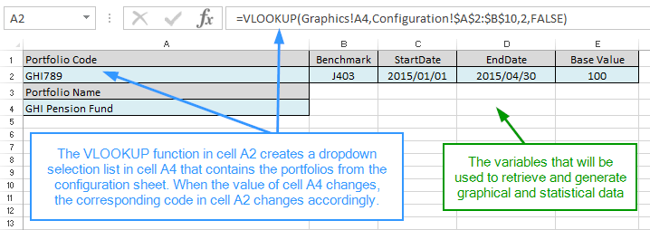
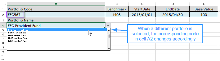
Use the drop down selector in cell A4 to choose different portfolios by name:
Create a TimeSeries call on a selected portfolio
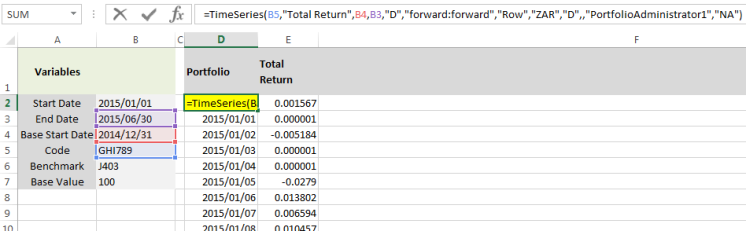
On the ‘data’ sheet, create a TimeSeries() function call that returns the total return for the selected portfolio between two dates. To make the sheet easier to read, create a block of variables that references those entered in the dashboard on the ‘graphics’ sheet:
Create a TimeSeries() function referencing the variables. Two columns are returned – value date and value (total return).
As calculations will be performed on these values, it could be useful to substitute any null values with zero by enclosing the TimeSeries function with the SubstituteArray() function as follows:
The Transform() function is used to add ‘1’ to the return values in order to calculate the cumulative returns:
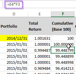
As the portfolio returns will be measured against an index, a base value is required to which to anchor both sets of return percentages in order to compare like with like. In this case 100 is used as a base value:
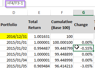
The daily change is also calculated and formatted as a percentage:
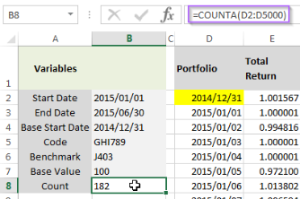
To create the total percentage return for the period, a record count is required:
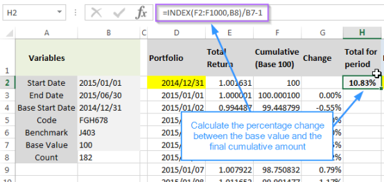
Calculate the total percentage return over the period for the portfolio
Use the Excel INDEX function and record count (182) to find the last cumulative amount in column F. Determine the percentage change between the base value (100) and the final cumulative amount:
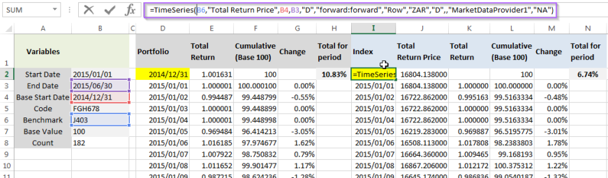
Repeat all steps above for the selected index
Repeat the exercise for the index by retrieving the total return price until the sheet looks as follows:
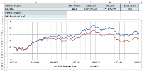
Create a graph and statistics to compare the performances
On the ‘graphics’ sheet under the variables ‘dashboard’, create a graph that uses the set of dates as the horizontal axis, and the cumulative values in column F of the ‘data’ sheet and column L of the ‘data’ sheet as series values:
| Dates | =Data!$D$2:INDEX(Data!$D$2:$D$5000,COUNTA(Data!$D$2:$D$5000),1) | Values in column D above, up to the value count |
| Fund performance | =Data!$F$2:INDEX(Data!$F$2:$F$5000,COUNTA(Data!$F$2:$F$5000),1) | Values in column F above, up to the value count |
| Index performance | =Data!$L$2:INDEX(Data!$L$2:$L$5000,COUNTA(Data!$L$2:$L$5000),1) | Values in column L above, up to the value count |
Calculate the comparative performance statistics per day
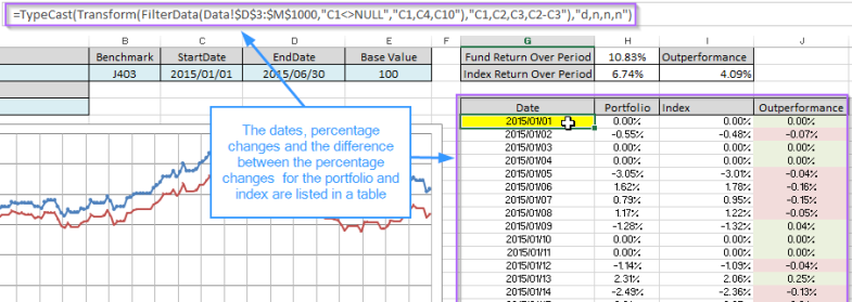
The goal is to create a table that lists the dates, the percentage change per day for the portfolio, the percentage change per day for the index, and the difference between the two.
First the relevant range of data is referenced from the ‘data’ sheet. The FilterData() function is used to filter any empty/null dates and to return the required columns from the range:
The Transform() function is used to display the three columns and to create a fourth column that subtracts the index percentages from the portfolio percentages to compare performance per day:
The TypeCast() function is used to ensure that the values are formatted correctly – in this instance a date and three numbers:
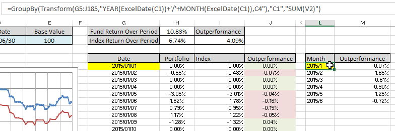
Calculate the comparative performance statistics per month
The Transform() function creates ‘Year/Month’ combinations from the dates in column G. The GroupBy() function is used to group and sum the outperformance column by ‘Year/Month’:
Create a graph showing the comparative performance statistics per month
The graph uses the Year/Month values as a horizontal axis and graphically represents the outperformance values:

The ‘graphics’ sheet forms the dashboard for inputting variables and displays the final report. Any of the values shaded in light blue can be changed and the statistics and graph will change accordingly: