How to calculate cumulative total returns
Calculating cumulative returns for a set of data that is variable in length is made easy using Quintessence.
See also:
Other use case examples:
- How to create a graphical return comparison in Excel using the Quintessence Excel® Addin functions
- How to build formulas in Excel using the Quintessence Excel® Addin functions
Example
Consider a TimeSeries() function for Entity Code “5010” that returns “Total Return” values between 2 May 2012 and 10 May 2012. It would be useful to calculate the cumulative total returns per day given a starting amount.
| TimeSeries function | |
| =TimeSeries(“5010″,”total return”,”2 May 2012″,”10 May 2012″,”td”,,”row”,,,,”MarketDataProvider1″) |
| Output | |
| 2012/05/02 | 0.001162255 |
| 2012/05/03 | -0.000805566 |
| 2012/05/04 | -0.003335329 |
| 2012/05/07 | -0.004588057 |
| 2012/05/08 | -0.012018702 |
| 2012/05/09 | -0.005395861 |
| 2012/05/10 | 0.01189494 |
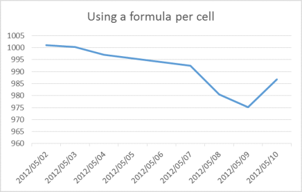
Using a formula per cell to calculate the cumulative total returns
One way to achieve the desired outcome would be to use a formula that is copied into successive cells. This example assumes a starting amount of 1000.
| A | B | C | D – Formula output | ||
| 1 | 1000 | Formula used in D | |||
|---|---|---|---|---|---|
| 2 | 2012/05/02 | 0.001162255 | 1001.162255 | =D1*(1+B2) | |
| 3 | 2012/05/03 | -0.000805566 | 1000.355753 | =D2*(1+B3) | |
| 4 | 2012/05/04 | -0.003335329 | 997.0192368 | =D3*(1+B4) | |
| 5 | 2012/05/07 | -0.004588057 | 992.4448559 | =D4*(1+B5) | |
| 6 | 2012/05/08 | -0.012018702 | 980.5169564 | =D5*(1+B6) | |
| 7 | 2012/05/09 | -0.005395861 | 975.226223 | =D6*(1+B7) | |
| 8 | 2012/05/10 | 0.01189494 | 986.8264808 | =D7*(1+B8) |
Graphical representation of the results
Using the Transform function to calculate the cumulative returns
Another way to achieve the desired result would be to use the Transform() utility function with Row Column syntax:
| TimeSeries function |
| =Transform(TimeSeries(“5010″,”total return”,”2 May 2012″,”10 May 2012″,”td”,,”row”,,,,”MarketDataProvider1″),”product(R(1)C(2):R(line)C(2)+1)*1000″) |
| A | B | C | D – Formula output | E – Transform function output |
| 1000 | ||||
| 2012/05/02 | 0.001162255 | 1001.162255 | 1001.162255 | |
| 2012/05/03 | -0.000805566 | 1000.355753 | 1000.355753 | |
| 2012/05/04 | -0.003335329 | 997.0192368 | 997.0192368 | |
| 2012/05/07 | -0.004588057 | 992.4448559 | 992.4448559 | |
| 2012/05/08 | -0.012018702 | 980.5169564 | 980.5169564 | |
| 2012/05/09 | -0.005395861 | 975.226223 | 975.226223 | |
| 2012/05/10 | 0.01189494 | 986.8264808 | 986.8264808 |
Graphical representation of the results
![]()
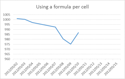
What happens when the number of records returned by the TimeSeries function increases?
In the two cases above, the results are identical. But now consider what happens when the number of records returned increases, for example the end date is changed to 15 May 2012.
| A | B | C | D – Formula output | E – Transform function output |
| 1000 | ||||
| 2012/05/02 | 0.001162255 | 1001.162255 | 1001.162255 | |
| 2012/05/03 | -0.000805566 | 1000.355753 | 1000.355753 | |
| 2012/05/04 | -0.003335329 | 997.0192368 | 997.0192368 | |
| 2012/05/07 | -0.004588057 | 992.4448559 | 992.4448559 | |
| 2012/05/08 | -0.012018702 | 980.5169564 | 980.5169564 | |
| 2012/05/09 | -0.005395861 | 975.226223 | 975.226223 | |
| 2012/05/10 | 0.01189494 | 986.8264808 | 986.8264808 | |
| 2012/05/11 | 0.004438005 | 991.2060216 | ||
| 2012/05/14 | -0.014041463 | 977.2880387 | ||
| 2012/05/15 | -0.000688366 | 976.6153071 |
As there are no additional formulas in column D, the new records are not evaluated. However, in column E, the Transform() function evaluates the total number of rows returned by the TimeSeries() function, so the new records are always evaluated, regardless of how many are returned. This is because the expression “product(R(1)C(2):R(line)C(2)+1)*1000” evaluates all rows in the TimeSeries output from the first row R(1) to the last row R(line).
Graphical representations of the results
![]()